GPT-2 —> Llama 3, One Improvement At A Time

If you happen to be one of the apparently 7m viewers (as of now) of Karpathy’s “Let’s build GPT: from scratch, in code, spelled out.”, and you also happen to be one of the minority that went through all of it, reasoned through it, and played with the code themselves, you might be surprised once it all clicks how simple it all is.

You might even ask: is this really all it takes? There must be more, right? Well, not to stomp on your much appreciated enthusiasm, and the entire premise of this blog, but… yeah, kinda. That is mostly all there is. If you take that simple architecture, do your data plumbing of the world’s knowledge and the skills you want your (Very Large!) Language Model to learn, and then spend most of your time scaling the training infrastructure using your very easy to afford datacenters, then yeah, you will go pretty far.

Attention huh. That really was the trick. It just works.

So.. is there nothing we can improve in the architecture itself? Why can’t I understand the modern LLM papers or most of the terminology people say? Are you lying to me??? Well well calm down. First of all, I appreciate that you are still asking, and the answer would be maybe… let’s not spoil too much. But if you come and think about what to improve with this magical attention-carried machine, I guess our thoughts would be… the stuff that’s not the attention part.

Psst, if you don’t know how GPT-2 works already, i recommend you go watch Karpathy’s GPT video and read a good visual blog like The Illustrated Transformer on the attention mechanism. It will make all this much easier to understand. If you did but feel rusty, don’t worry, we will accidentally talk about the intuition of each part while going through it anyways!

So say we have this sentence

Mary found a shiny rock

and we are trying to guess the next word. It might sound tiny, but it already requires a lot. For the model to guess the next word better than random, it has to learn from many failed guesses. It has to learn representations where similar words live near each other, learn some knowledge of the world in its weights, learn how related words and concepts interact, and do all of that across many layers that slowly build more abstract features. By the end, the model is kinda reasoning, even if all it is technically doing is trying to guess the next token.

So what matters is this: take the words in as vectors, embed them in a sensible space, let each word look at the other words in the context, and then mix in the useful information. If shiny matters for rock, the representation for rock should be able to carry some of that information forward. Then when the next layer touches that token, it is not just seeing rock alone anymore. It is seeing rock, but with the relevant context baked into it. This scales very well, and across many layers the model learns to care about different kinds of things.

Quick GPT-2 Refresher

Okay I know that my previous sentences packed a lot, basically the entire GPT-2 block hiding in one paragraph. So let’s slow it down and refresh how GPT-2 works.

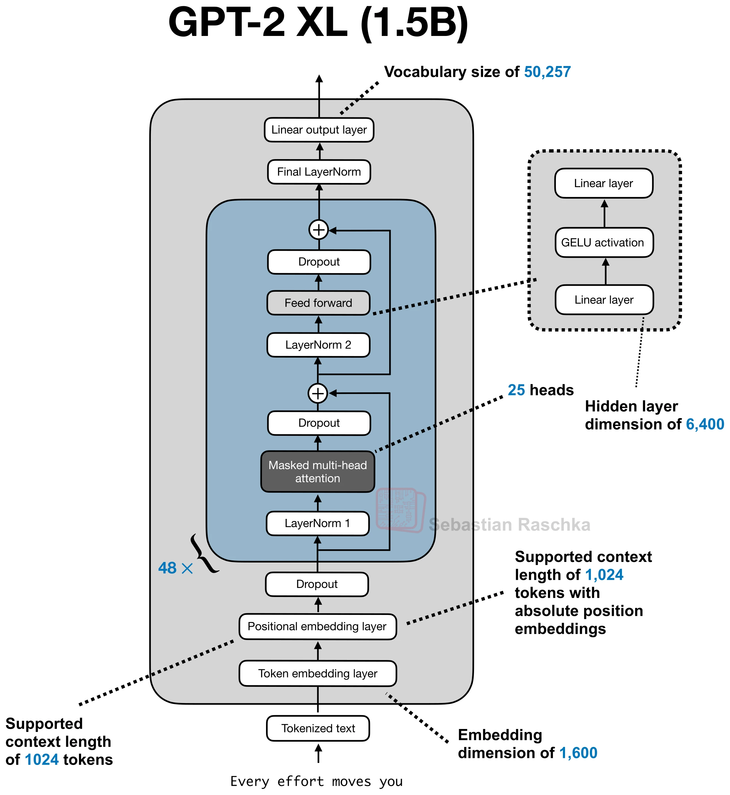
First, we do not feed the sentence into the model as raw text. GPT-2 uses a byte-level BPE tokenizer, which is basically a middle ground between character-level and word-level. We are not forced to treat every character separately, but we also do not need one giant vocabulary entry for every possible word.

So a sentence like:

Mary found a shiny rock

gets chopped into tokens. For common words, this might look almost word-like:

Mary, found, a, shiny, rock

and for weirder words, the tokenizer might split them into smaller chunks. The important thing is that the model does not see “words” exactly. It sees token IDs.

Then each token ID goes through an embedding table. You can think of this table as a giant lookup table:

x = token_embedding[token_id]

So now every token becomes a vector. At the beginning these vectors are kinda dumb, but through training the model keeps adjusting them until tokens that behave similarly start getting useful representations.

Then attention asks: for each token, what other tokens should I look at?

This is where the query, key, and value thing comes in. For every token vector x, the model creates three new vectors by multiplying it with three learned matrices:

q = x @ Wq
k = x @ Wk
v = x @ Wv

This is one of those things that sounds more mysterious than it is. We are taking the same token representation and making three different “views” of it.

The query is the token asking a question: “what kind of information am I looking for?”

The key is the token advertising itself: “what kind of thing am I?”

The value is the actual information the token will pass along if another token decides to care about it.

So if we are updating the representation for rock, the query of rock gets compared with the keys of the previous tokens. It asks something like: should I care about Mary? should I care about found? should I care about shiny?

The comparison is just a dot product:

score = q_rock @ k_other

If the query of rock lines up well with the key of shiny, that score becomes large. After we do this against all the earlier tokens, we pass the scores through a softmax, and now they become attention weights.

Then we use those weights to mix the values:

new_rock = sum(attention_weight_i * value_i)

So the representation at rock is no longer just rock. It is rock, plus whatever context attention decided was useful. In this case, maybe shiny gets mixed in strongly, because it modifies the noun. Maybe Mary matters less for this local meaning.

That updated vector goes back into the residual stream, then the MLP processes it locally, and then the next layer gets to do the same thing again with a richer version of the token.

And this is why attention is so powerful. It lets every token build a context-aware version of itself.

RoPE

One thing that I conveniently skipped though, is that we need the model to know that “Mary found a shiny rock” is not the same thing as “rock shiny a found Mary.” In GPT-2 this is handled with learned positional embeddings. Each position gets its own learned vector, and we add that to the token embedding before attention. So now the model knows not just what the word is, but where it sits in the sequence. For example, Mary might be at position 0, while shiny might be at position 3.

This Gives the model order information, and over training it can learn some relative patterns from it, to better understand, given some word how far and in what direction is the other word.

The same kind of relationship between words can happen in many different places in a sentence. An adjective can be right next to the noun it modifies, or a bit farther away. A pronoun can refer to something a few tokens back, or many tokens back. Structurally these are very similar kinds of relationships, but with absolute positional embeddings the model is only told the raw positions of each token, and it has to learn for itself that these patterns are “the same kind of thing” happening at different locations.

as you might guess attention really cares about that kind of relationship between tokens, but notice something, we aren’t telling it that relationship between tokens directly, and it does feel awkward having it try to learn it from the absolute positional embeddings.

Soo hmmm i see how it cares about that, could we not give it that more directly instead of hoping it painfully infers it from absolute position vectors? Well well, that’s a great question and that is basically the intuition behind something called RoPE, or Rotary Position Embedding. So then the question becomes: how do we build that into attention?

To figure out how to do that, we should look at where attention even decides relevance in the first place. A token does not attend to another token by magic. It happens through the query-key dot product. The query of the current token is compared against the keys of the other tokens, and from that we get the attention weights. So if we want relative position to affect attention more directly, then the most natural place to inject it is not somewhere random in the block, but right there in the queries and keys themselves.

Now we want something a bit specific. We want to change queries and keys depending on position, but not in a way that destroys what they already mean. They still need to carry semantic information. We just want their interaction to now also reflect position more naturally. So instead of adding yet another position vector from the outside, what if we transformed the query and key themselves depending on where they are in the sequence? And now a cute idea appears: rotation. Why rotation? Because rotation changes the direction of a vector without just blowing up its size or mangling it in some ugly way. So the token can still keep its “meaning” information, but the way it lines up with other tokens in the dot product now changes with position. And that is the big jump in RoPE. We are no longer saying, “here is position 17, please remember it.” We are saying, “let position change how queries and keys compare to each other.”

Okay bro i hear you but why does rotating both actually give relative position, how does that happen. Well think about what the dot product is even doing. It is basically asking how lined up two vectors are? If two vectors are rotated by the same amount, they still line up almost the same, but if one is rotated different from the other, their alignment changes. So once we rotate the query and key based on where they are in the sequence, the attention scores start caring less about their raw absolute position by themselves, and more about the difference between these positions, and that difference is the thing we wanted all along! So in a way, RoPE is sneaky. We are not explicitly writing down “this token is 4 words away from that token.” Instead, we rotate both vectors according to position, and then the dot product naturally turns that into something that depends on how far apart they are. That is why it feels so much cleaner than just slapping absolute position vectors on from the outside. You might now have the intuition behind it, which is really what matters. But if you are still wondering on how do we actually implement all this. Well it starts to get a little bit mathy, although note that all that math is just us trying to make what we described happen, and that math on it’s essence actually simple. Now our key and query are actually not some cute 2D arrows, they are in fact quite high dimension, and when we do something in the realm of ML, we wanna both figure out the math to do it, and the trick to do it quickly with little memory. So how do we do it?

Now we just need to make that same little 2D rotation idea work inside a high-dimensional vector. We do that by taking the dimensions in pairs. So instead of thinking of the query as one giant blog of numbers, we think of it as many tiny 2D subspaces sitting next to each other. The first two dimensions are on little plane, then next two are another, and so on. Then for each pair we do the exact same rotation trick we just talked about. So if a query has dimensions like:

q = [q0, q1, q2, q3, q4, q5, ...]

we group them like:

• (q0, q1)
• (q2, q3)
• (q4, q5)

and rotate each pair.

Now of course if we rotated every pair by the exact same amount, that would be too simple. We want the model to be able to notice both short range and long range relationships. So different pairs rotate at different speeds. Some pairs rotate slowly, which helps track broader positional structure, and some rotate faster, which helps capture finer local differences. In the dot product, this means some pairs are very sensitive to small changes in relative position, while others change more slowly and can still track broader positional relationships. So instead of attention getting one single crude positional signal, it gets many little positional signals at different scales.

This is very similar in spirit to the old sinusoidal positional encoding idea used in the original transformer, where different dimensions carry positional information at different frequencies.

So for a token at position p, each pair gets rotated by an angle that depends on:

• the token position p
• and the frequency assigned to that pair

So the angle is basically:

$$\theta_{p,j} = p \cdot \text{frequency}_j$$

and then we apply a normal 2D rotation:

$$\begin{bmatrix} x' \\ y' \end{bmatrix} = \begin{bmatrix} \cos(\theta) & -\sin(\theta) \\ \sin(\theta) & \cos(\theta) \end{bmatrix} \begin{bmatrix} x \\ y \end{bmatrix}$$

And that my friend is the heart of RoPE.

We do this to the query and the key, using the token’s position, before taking the attention dot product. Also you might notice that we are only rotating the queries and keys and not the values, why is that? Well that is because the thing we want to change is the attention score itself, the part where tokens decide how much they care about each other. That score comes from query-key interaction, so that is exactly where RoPE belongs.

Now if we wanted to do this in the dumbest possible way, we could imagine building an actual little rotation matrix for every pair of dimensions at every position and applying it directly. That would work in theory, but it would be silly and slow. Instead, we notice that a 2D rotation only really needs cos(angle) and sin(angle). So in practice we precompute the cosine and sine values for each position and each pair of dimensions, and then apply the rotation with a bit of simple elementwise arithmetic.

That is why in code RoPE often looks much simpler than it sounds in words. You usually see something like:

• split even and odd dimensions
• treat each pair as a tiny 2D vector
• build the rotated version by swapping and negating one side
• multiply by cos
• multiply by sin
• add them together

and boom, you have done the rotation.

Ok cool, but how does that look like in code?

Surprisingly small.

We only need three little pieces:

• a way to rotate each pair of dimensions
• a way to precompute the cosine and sine values for each position
• and a way to apply them to the query and key

The first one is the smallest and also the weirdest looking at first:

def rotate_half(x):
    x_even = x[..., ::2]
    x_odd  = x[..., 1::2]
    x_rot = torch.stack((-x_odd, x_even), dim=-1)
    return x_rot.flatten(-2)

At first this looks random, but it is really just the 90-degree rotation part of the 2D trick. Remember, we grouped the dimensions in pairs:

• (x0, x1)
• (x2, x3)
• (x4, x5)

If one pair is (a, b), then rotating it in 2D involves mixing those two numbers together. A very important part of that rotation is turning:

• (a, b) into (-b, a)

and that is exactly what rotate_half is doing across every pair of dimensions in the vector. So rotate_half is not the full RoPE rotation by itself. It is just the little helper that gives us the “swapped and negated” part we need.

The next piece is building the angles we want to rotate by:

def build_rope_cache(seq_len, head_dim, device=None, base=10000, dtype=torch.float32):
    assert head_dim % 2 == 0, "RoPE needs an even head_dim"

    half_dim = head_dim // 2
    positions = torch.arange(seq_len, device=device, dtype=torch.float32)

    freqs = 1.0 / (
        base ** (torch.arange(half_dim, device=device, dtype=torch.float32) / half_dim)
    )

    angles = torch.outer(positions, freqs)
    angles = torch.repeat_interleave(angles, 2, dim=-1)

    cos = angles.cos()[None, None, :, :].to(dtype=dtype)
    sin = angles.sin()[None, None, :, :].to(dtype=dtype)
    return cos, sin

This part is doing two jobs. First, it makes a list of token positions:

• 0
• 1
• 2
• …

Then it makes a list of frequencies, one for each pair of dimensions. That is the “different pairs rotate at different speeds” part. Some pairs rotate faster, which makes them more sensitive to local positional changes. Some rotate slower, which gives a broader sense of position. Then we combine them with:

$$\text{angle}_{p,j} = \text{position}_p \cdot \text{frequency}_j$$

So for every token position, and for every pair of dimensions, we get the angle that pair should rotate by. After that we just take the cosine and sine of those angles, because that is all a 2D rotation really needs.

And now the actual rotation ends up being surprisingly small:

def apply_rope(x, cos, sin):
    return x * cos + rotate_half(x) * sin

This line is the whole thing cashing out. If you remember the normal 2D rotation:

$$x' = x\cos(\theta) - y\sin(\theta)$$ $$y' = x\sin(\theta) + y\cos(\theta)$$

this function is just doing that in vectorized form across all the little dimension pairs at once.

• x * cos gives one part
• rotate_half(x) * sin gives the other part
• add them together, and you get the rotated query or key

Now we only need to use it in the right place. As we concluded logically before we do not apply RoPE to the raw token embeddings, and we do not apply it to the values. We apply it to the queries and keys, right before attention scores are computed.

q = self.Wq(x)
k = self.Wk(x)

q = q.view(bsz, seqlen, self.n_heads, self.head_dim).transpose(1, 2)
k = k.view(bsz, seqlen, self.n_kv_heads, self.head_dim).transpose(1, 2)

cos, sin = build_rope_cache(seqlen, self.head_dim, device=x.device, dtype=q.dtype)

q = apply_rope(q, cos, sin)
k = apply_rope(k, cos, sin)

That is the full idea in code. First we project into queries and keys. Then we reshape them into attention heads. Then we build the cosine and sine values for the positions in this sequence. Then we rotate both q and k. And only after that do we let them meet in the dot product that produces the attention scores. So the final effect is exactly what we wanted from the beginning and instead of telling a token where it is, we now successfully are changing how tokens compare to each other inside attention itself.

Pheww, we dove a bit into the math there, but as you saw, fundamentally all of it was pretty logical. We did not have to make some giant weird leap. Still, theory is theory. The important question is always: did this actually help in practice?

On the same TinyStories setup, with the same small model shape and training budget, the RoPE version reached a validation loss of 2.3748, compared to 2.5400 for the learned absolute positional embedding baseline.

Model	Position / block change	Validation loss
GPT-2-style baseline	learned absolute positional embeddings	2.5400
GPT-2 + RoPE	RoPE instead of learned absolute positional embeddings	2.3748
Llama-style dense mini	RoPE + RMSNorm + SwiGLU	2.2722

That is a pretty nice result for such a surgical change. We did not redesign the whole block, we did not change the training setup, and we did not suddenly make the model bigger. We only changed how position enters attention, and it worked better. And I think the intuition here makes sense too. With learned absolute positional embeddings, the model has to work harder to back its way into the relative relationships attention really cares about. With RoPE, we are giving attention something much closer to the thing it wanted in the first place. So in this short training run, the model seems to pick up that structure more easily.

Normalization

Ok cool position feels less awkward now. Now continuing on with our hunt for the next piece to improve, one of the places we can try to look at next is the LayerNorm we had in GPT-2.

Why do we normalize in the first place?

Every layer keeps writing into the residual stream. Attention writes into it, then the MLP writes into it, then the next block does the same thing again. If we just keep doing that with no control, the scale of the activations can drift around and training becomes annoying. So normalization is basically a way of keeping the stream in a sane numerical range.

GPT-2 uses LayerNorm. LayerNorm does two things:

• it subtracts the mean, which recenters the activations
• it divides by the standard deviation, which rescales them

$$\mu = \frac{1}{d}\sum_{i=1}^{d} x_i, \qquad \sigma^2 = \frac{1}{d}\sum_{i=1}^{d}(x_i - \mu)^2$$ $$\mathrm{LayerNorm}(x)_i = \gamma_i \frac{x_i - \mu}{\sqrt{\sigma^2 + \epsilon}} + \beta_i$$

So you can think of LayerNorm as saying: “let me recenter this vector and also keep its scale under control.” But now a question might appear: do we really need both parts?

Well… we can try simply removing either the re-centering or the rescaling and see how it will affect us.

so trying out the recentering part only

$$\mathrm{CenterOnly}(x)_i = x_i - \mu$$

and then run our experiment. It is a lot worse! Almost like running without useful normalization. Ok so how about the opposite since the rescaling is so important. Instead of subtracting the mean and then normalizing, we basically keep the “make sure this vector stays at a sane scale” part, and drops the explicit recentering part

$$\mathrm{RMS}(x) = \sqrt{\frac{1}{d}\sum_{i=1}^{d}x_i^2 + \epsilon}$$ $$\mathrm{RMSNorm}(x)_i = \gamma_i \frac{x_i}{\mathrm{RMS}(x)}$$

Interesting!! it works just as well, and we are doing a teeny tiny bit less computation as well, neat! And this is actually what Llama 3 uses.

Ok so let’s incorporate this into the code as well

class RMSNorm(nn.Module):
    def __init__(self, dim, eps=1e-5):
        super().__init__()
        self.eps = eps
        self.weight = nn.Parameter(torch.ones(dim))

    def forward(self, x):
        rms = torch.rsqrt(x.pow(2).mean(dim=-1, keepdim=True) + self.eps)
        return (x * rms) * self.weight

This code is doing exactly what we said:

• square the activations
• average them across the feature dimension
• take the reciprocal square root
• multiply the original vector by that scale
• then apply a learned per-dimension weight

So compared to LayerNorm, the main thing missing is the mean subtraction.

This is one of those places where the idea is partly intuitive and partly empirical. The intuition is that the residual stream mostly needs stable scale. The empirical result, from the RMSNorm paper and from modern Llama-style models, is that dropping the recentering still works well.

SwiGLU

Cool position is now cleaner, normalization is simpler. what should be the next piece to hunt, a possible one we haven’t touched yet is the MLP.

So after the tokens communicate with each other in attention, and the relevant context gets mixed into each token, the result goes to the MLP. Attention is where tokens talk to each other. The MLP is where each token gets processed locally after that conversation.

A useful way to think about it is: attention gathers the context, and the MLP decides what to do with that context. A lot of feature transformations, and a lot of the factual-looking behavior people talk about in language models, seem to live in these feedforward weights. Not all of the model’s knowledge is magically inside the MLP, but it is definitely one of the main places worth poking.

in GPT-2 it’s pretty simple:

x = self.gelu(self.fc1(x))
x = self.fc2(x)

This is basically: expand, apply one nonlinearity, compress. And it works. But after attention, the token representation is carrying a messy mixture of information: syntax, reference, local word meaning, maybe some longer-range clue. Treating all of that with one big GELU transformation feels a bit blunt.

So how can the MLP be more selective?

One simple way to make something selective is to give it a gate! instead of making one hidden representation and passing it through GELU, make two hidden representations:

• one path proposes features
• the other path decides how much of these features pass through

That is the whole idea behind a gated MLP.

So we want something shaped like:

$$h = \text{candidate\_features} \odot \text{gate}$$

Now question becomes what should the gate be?

The simplest version would be to make the gate with a sigmoid, because sigmoid naturally gives us something gate-like: numbers between 0 and 1. So you can imagine:

candidate = W_up(x)
gate = sigmoid(W_gate(x))
hidden = candidate * gate

Now one path proposes features, and the other path decides how much of each feature gets through.

But we already had a smooth activation in the GPT-2 MLP: GELU. So another natural idea is: what if the gate used GELU instead of sigmoid?

$$h = W_{\mathrm{up}}(x) \odot \mathrm{GELU}(W_{\mathrm{gate}}(x))$$

This is called GEGLU.

And then comes the Llama-style choice: instead of using GELU for the gate, use SiLU, also called Swish:

$$\mathrm{SiLU}(x) = x \cdot \sigma(x)$$

So the gated MLP becomes:

$$h = W_{\mathrm{up}}(x) \odot \mathrm{SiLU}(W_{\mathrm{gate}}(x))$$

And that is SwiGLU. Which is what we use in our Llama 3 architecture for the MLP.

And here is the full code for it

class SwiGLU(nn.Module):
    def __init__(self, n_embed, hidden_dim=None, dropout=0.1, bias=False):
        super().__init__()
        hidden_dim = hidden_dim or (4 * n_embed)

        self.w1 = nn.Linear(n_embed, hidden_dim, bias=bias)  # gate
        self.w3 = nn.Linear(n_embed, hidden_dim, bias=bias)  # candidate
        self.w2 = nn.Linear(hidden_dim, n_embed, bias=bias)  # project back
        self.dropout = nn.Dropout(dropout)

    def forward(self, x):
        x = F.silu(self.w1(x)) * self.w3(x)
        x = self.w2(x)
        return self.dropout(x)

So compared to GPT-2, this is not just “replace GELU with SiLU.” The real change is that we split the hidden computation into two paths:

• w3(x) proposes candidate features
• silu(w1(x)) decides how much of those features should pass through
• w2 projects the result back down

So the MLP becomes more selective. After attention gathers context, the MLP can decide which local features are actually useful for this token.

At this point, we have covered the first modeling-side chunk of the path from a GPT-2-style block toward a Llama-style one:

• position is no longer pasted on from the outside; RoPE moves it into attention
• normalization is simpler; RMSNorm keeps the scale control and drops explicit recentering
• the MLP is more selective; SwiGLU turns the feedforward block into a gated computation

There are still important Llama-style pieces left, especially split Q/K/V, GQA, and KV cache. But those come from a slightly different pressure. LLMs are not just trained, they are deployed to generate one token at a time at scale. So from here the questions become more systems-flavored: how do we reduce memory movement, shrink the KV cache, and make inference cheaper without losing performance?

So I will stop this part here. If you are following along in code, the best thing you can do now is train the small GPT-2 baseline, replace one piece at a time, and actually watch what changes. The point is not to memorize the names RoPE, RMSNorm, and SwiGLU. The point is to understand the annoyance each one is answering.

Resources

• Andrej Karpathy, “Let’s build GPT: from scratch, in code, spelled out.”
• Jay Alammar, “The Illustrated Transformer”
• Sebastian Raschka, “LLM Architecture Gallery”
• Vaswani et al., “Attention Is All You Need”
• Su et al., “RoFormer: Enhanced Transformer with Rotary Position Embedding”
• Zhang and Sennrich, “Root Mean Square Layer Normalization”
• Shazeer, “GLU Variants Improve Transformer”
• Meta, “Introducing Meta Llama 3”
• Meta Llama 3 model card